Courses·Training Fundamentals·7 min read

Backpropagation and Gradient Descent

Backpropagation is the algorithm that computes how much each parameter in a neural network contributed to the prediction error, enabling gradient descent to systematically adjust billions of parameters toward better predictions.

One-Line Summary: Backpropagation is the algorithm that computes how much each parameter in a neural network contributed to the prediction error, enabling gradient descent to systematically adjust billions of parameters toward better predictions.

Prerequisites: Basic calculus (derivatives, chain rule), understanding of neural network layers, the concept of a loss function, matrix multiplication, basic understanding of transformer architecture.

What Is Backpropagation?

Imagine you are managing a factory with a thousand machines arranged in a pipeline. The final product comes out defective. You need to figure out which machines, and which settings on those machines, contributed to the defect -- and by how much. If you could trace the defect backward through every machine in the pipeline and compute each machine's contribution, you could adjust every setting simultaneously to improve the product.

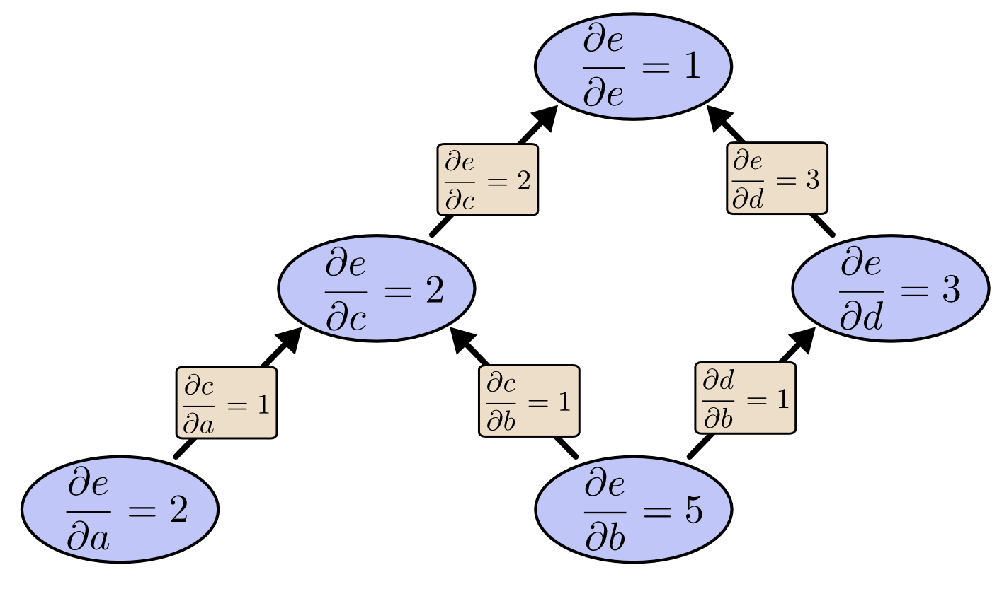Computational graph of a neural network showing the forward pass computing activations and the backward pass propagating gradients via the chain rule Source: Chris Olah -- Calculus on Computational Graphs: Backpropagation

That is backpropagation. It is the algorithm for computing gradients -- the direction and magnitude of change needed for every parameter in the network to reduce the loss. Once you have these gradients, gradient descent uses them to actually update the parameters.

Backpropagation is not a learning algorithm itself. It is a gradient computation algorithm. Combined with an optimizer like Adam, it forms the complete learning system.

How It Works

flowchart TD
    L1["how the chain rule decomposes the total gr"]
    L2["local gradient products at each layer"]
    L1 --> L2

The Forward Pass

Before gradients can be computed, the model must process input and produce a prediction:

Input tokens are converted to embeddings.
Embeddings pass through $N$ transformer layers, each applying self-attention and feed-forward operations.
The final layer produces logits over the vocabulary.
Softmax converts logits to probabilities.
Cross-entropy loss is computed against the true next tokens.

Every intermediate computation is recorded on a computational graph -- a directed acyclic graph (DAG) where nodes represent operations and edges represent data flow. This graph is essential for the backward pass.

The Chain Rule

The mathematical foundation of backpropagation is the chain rule of calculus. If a loss $L$ depends on a parameter $w$ through a chain of functions:

$L = f (g (h (w)))$

then:

$\frac{\partial L}{\partial w} = \frac{\partial f}{\partial g} \cdot \frac{\partial g}{\partial h} \cdot \frac{\partial h}{\partial w}$

In a neural network, the "chain" can be hundreds of operations long. Backpropagation applies the chain rule efficiently by computing gradients layer-by-layer from the output back to the input.

The Backward Pass

Starting from the loss $L$ :

Compute $\frac{\partial L}{\partial logits}$ : For cross-entropy with softmax, this is simply $\overset{y}{^} - y$ (predicted minus true distribution).
Propagate through the output projection: Compute gradients with respect to the final linear layer's weights and biases, and with respect to its input (the transformer's output).
Propagate through each transformer layer in reverse order: For each layer $l = N, N - 1, \dots, 1$ :
- Gradients flow through the layer normalization.
- Gradients flow through the feed-forward network (two linear layers with an activation).
- Gradients flow through the residual connection (this simply copies the gradient).
- Gradients flow through the multi-head self-attention (computing gradients for Q, K, V projections and the attention weights).
- Gradients flow through another layer normalization and residual connection.
Propagate through the embedding layer: Compute gradients for the token embedding and positional embedding matrices.

At every step, two things are computed: (a) the gradient with respect to the layer's parameters (for the optimizer to use), and (b) the gradient with respect to the layer's input (to pass to the preceding layer).

Gradient Descent Update Rule

Once all gradients are computed, the simplest update rule (vanilla gradient descent) is:

$θ_{t + 1} = θ_{t} - η \cdot \nabla_{θ} L$

where $η$ is the learning rate and $\nabla_{θ} L$ is the gradient of the loss with respect to all parameters. In practice, LLMs use sophisticated optimizers like AdamW rather than vanilla gradient descent.

The Computational Graph in Practice

Modern deep learning frameworks (PyTorch, JAX) build the computational graph automatically during the forward pass (automatic differentiation). When you call loss.backward() in PyTorch, the framework traverses this graph in reverse, applying the chain rule at each node. This is why every operation in a neural network must be differentiable -- the chain rule requires that every link in the chain has a well-defined derivative.

Gradient Flow Through Transformer Layers

Transformers have specific properties that affect gradient flow:

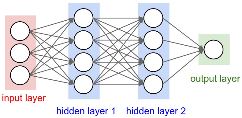Neural network forward pass and backward pass showing how gradients flow back through layers Source: Stanford CS231n – Neural Networks

Residual connections: These create "gradient highways" that allow gradients to flow directly from the loss to early layers without being multiplied through every intermediate operation. The residual connection means the gradient at layer $l$ is:

$\frac{\partial L}{\partial x _{l}} = \frac{\partial L}{\partial x _{l + 1}} + \frac{\partial L}{\partial x _{l + 1}} \cdot \frac{\partial f _{l} ( x _{l} )}{\partial x _{l}}$

The additive term prevents gradients from vanishing, which was a critical problem in pre-transformer architectures (RNNs, LSTMs).

Layer normalization: Normalizes gradients at each layer, preventing them from growing or shrinking uncontrollably.
Attention mechanism: Gradients flow through the softmax attention weights, meaning that tokens with high attention scores receive stronger gradient signals. The attention gradient involves:

$\frac{\partial L}{\partial Q} = \frac{\partial L}{\partial Attn} \cdot K^{T}, \frac{\partial L}{\partial K} = \frac{\partial L}{\partial Attn}^{T} \cdot Q$

Memory Requirements

Backpropagation requires storing all intermediate activations from the forward pass (they are needed to compute gradients). For a large transformer, this can consume enormous memory. A model with 70 billion parameters might require:

See also the visual explanation of gradient flow through residual connections at: Jay Alammar -- The Illustrated Transformer -- shows how skip connections in transformers create gradient highways that prevent vanishing gradients.

Parameters: ~140 GB (in FP16/BF16)
Optimizer states: ~560 GB (Adam stores 2 additional copies per parameter)
Activations: Hundreds of GB, depending on batch size and sequence length

This is why techniques like gradient checkpointing (recomputing activations instead of storing them) and model parallelism are essential.

Why It Matters

Without backpropagation, training neural networks of any meaningful size would be computationally infeasible. Before backpropagation was widely adopted (popularized by Rumelhart, Hinton, and Williams in 1986), there was no efficient way to compute gradients for multi-layer networks. The alternative -- numerical differentiation (perturbing each parameter individually) -- would require a separate forward pass for each of the billions of parameters, making it astronomically slower.

Backpropagation reduces the cost of computing all gradients to roughly 2-3 times the cost of a single forward pass, regardless of the number of parameters. This efficiency is what makes training billion-parameter models feasible.

Key Technical Details

Compute cost: The backward pass is approximately 2x the cost of the forward pass (it must compute gradients for both parameters and activations at each operation).
Memory cost: Storing activations for backpropagation is often the dominant memory cost during training, exceeding the memory needed for the parameters themselves.
Gradient accumulation: Gradients can be accumulated across multiple forward-backward passes before performing a parameter update, effectively simulating larger batch sizes.
Gradient checkpointing: Trades compute for memory by not storing some intermediate activations and recomputing them during the backward pass.
Mixed precision: Gradients are often computed in FP16/BF16 but accumulated in FP32 for numerical stability.
Non-differentiable operations: Discrete operations (argmax, sampling) cannot be backpropagated through, which is why techniques like the straight-through estimator or policy gradient methods (REINFORCE) are needed for reinforcement learning from human feedback.

Common Misconceptions

"Backpropagation is a learning algorithm." It is a gradient computation algorithm. The learning algorithm is gradient descent (or Adam, etc.) that uses those gradients to update parameters.
"Backprop is biologically plausible." The brain almost certainly does not implement backpropagation. The requirement to propagate error signals backward through every layer, using the exact same weights as the forward pass, has no known biological mechanism.
"Gradients tell you the optimal parameter values." Gradients only indicate the local direction of improvement. They say nothing about the global optimum. Neural network loss landscapes are highly non-convex with many local minima and saddle points.
"All parameters receive equal gradient signal." In practice, different parts of the network receive very different gradient magnitudes, which is why adaptive optimizers like Adam are necessary.

Connections to Other Concepts

cross-entropy-loss.md: The function whose gradients backpropagation computes.
adam-optimizer.md: The algorithm that uses the computed gradients to update parameters.
gradient-clipping.md: Applied to gradients after backpropagation to prevent instability.
mixed-precision-training.md: Affects how gradients are computed and stored.
gradient-checkpointing.md: A memory optimization technique that modifies how backpropagation stores intermediate activations.
residual-connections.md: Architectural feature that directly improves gradient flow.