Courses·Foundational Architecture·7 min read

Autoregressive Generation

Autoregressive generation is the process by which LLMs produce text one token at a time, feeding each newly generated token back as input for predicting the next, creating a sequential feedback loop that is both the source of their generative power and their primary inference bottleneck.

One-Line Summary: Autoregressive generation is the process by which LLMs produce text one token at a time, feeding each newly generated token back as input for predicting the next, creating a sequential feedback loop that is both the source of their generative power and their primary inference bottleneck.

Prerequisites: Understanding of the Transformer decoder, causal (masked) attention, the softmax output layer, and the concept of conditional probability.

What Is Autoregressive Generation?

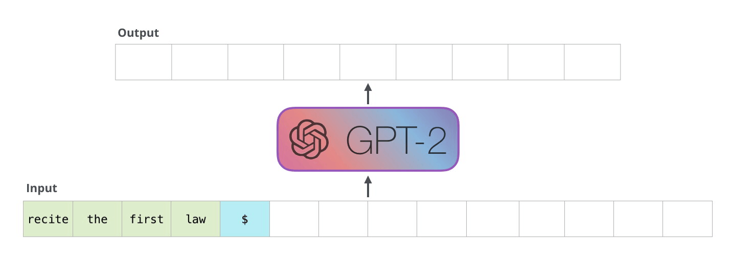
The term "autoregressive" means "self-feeding" -- the model's own outputs become its future inputs. Imagine a storyteller who writes one word, reads back everything written so far (including the new word), then writes the next word. This continues until the story is complete.

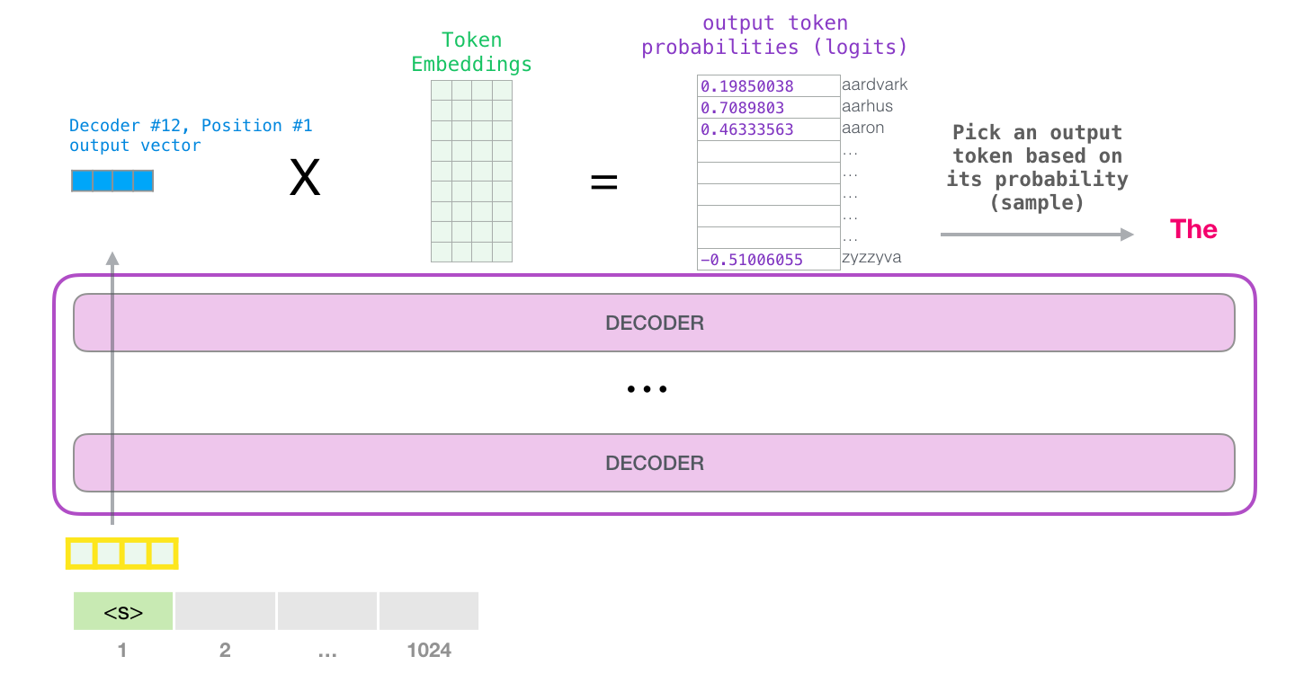Autoregressive generation process showing the two phases: prefill (processing the full prompt in parallel) and decode (generating tokens one at a time with the KV cache growing at each step) Source: The Illustrated GPT-2 -- Jay Alammar

More formally, the model factors the probability of a sequence as a product of conditional probabilities:

$P (t_{1}, t_{2}, \dots, t_{n}) = \prod_{i = 1}^{n} P (t_{i} ∣ t_{1}, t_{2}, \dots, t_{i - 1})$

At each step, the model computes a probability distribution over the entire vocabulary (typically 32,000 to 128,000+ tokens), selects one token from this distribution, appends it to the sequence, and repeats. Generation terminates when the model produces a special end-of-sequence (EOS) token or reaches a maximum length.

How It Works

GPT-2 generating text token by token, showing how each newly generated token is fed back as input and the model produces a probability distribution over the vocabulary at each step Source: The Illustrated GPT-2 -- Jay Alammar

The Two Phases: Prefill and Decode

Modern LLM inference has two distinct computational phases:

flowchart LR
    S1["GPT-2 autoregressive generation"]
    S2["each new token being fed back as input for"]
    S1 --> S2

Phase 1: Prefill (Processing the Prompt)

When you send a prompt to an LLM, the entire prompt is processed in a single forward pass. All tokens in the prompt are fed through the model simultaneously (just like during training). The model:

Processes all prompt tokens through every layer in parallel.
Computes and stores the keys and values for every token at every layer (the KV cache).
Produces logits for the next token after the prompt.

This phase is compute-bound: it involves dense matrix multiplications over the full prompt length. A 1000-token prompt is processed in roughly the same wall-clock time as a 100-token prompt (on modern hardware with sufficient parallelism), though it requires more computation.

Phase 2: Decode (Generating Tokens)

After prefill, the model generates one new token at a time:

The new token's embedding is fed through the model (just one token, not the full sequence).
At each attention layer, the new token's query attends to all cached keys and values (from the prompt and all previously generated tokens).
New key and value vectors for this token are computed and appended to the KV cache.
The model produces logits, a token is selected, and the process repeats.

This phase is memory-bandwidth-bound: each step requires reading all model weights and the entire KV cache from GPU memory, but only computes a single token's forward pass. This is extremely inefficient in terms of hardware utilization, which is why generation is much slower per token than prefill.

The KV Cache

The KV cache is the critical optimization that makes autoregressive generation practical. Without it, generating token $t_{n}$ would require reprocessing all $n - 1$ previous tokens from scratch -- an $O (n^{2})$ total cost for generating $n$ tokens.

With the KV cache:

During prefill, keys and values for all prompt tokens are computed and stored.
During each decode step, only the new token's keys and values are computed and appended.
The cached keys and values are reused in every subsequent step's attention computation.

This reduces the decode phase from $O (n^{2})$ to $O (n)$ total computation (each step is $O (1)$ in terms of the new token's computation, though $O (n)$ in terms of the attention over cached tokens).

KV cache memory: For a model with $L$ layers, $h$ heads, head dimension $d_{k}$ , and sequence length $n$ , the KV cache requires:

$KV cache memory = 2 \times L \times h \times d_{k} \times n \times bytes per element$

For a 70B-parameter model with 80 layers, GQA with 8 KV heads, $d_{k} = 128$ , and a 4096-token sequence in float16:

$2 \times 80 \times 8 \times 128 \times 4096 \times 2 bytes \approx 1.3 GB$

This grows linearly with sequence length and becomes a major constraint for long-context inference.

Token Selection (Decoding Strategies)

After the model produces logits for the next token, how is the actual token chosen?

Greedy decoding: Always pick the highest-probability token. Deterministic but can produce repetitive, boring text.
Top-k sampling: Sample from only the $k$ most probable tokens. Controls randomness by limiting options.
Top-p (nucleus) sampling: Sample from the smallest set of tokens whose cumulative probability exceeds $p$ . Adapts dynamically to the confidence of the distribution.
Temperature sampling: Divide logits by a temperature $T$ before softmax. $T < 1$ sharpens the distribution (more deterministic); $T > 1$ flattens it (more random).
Beam search: Maintain $k$ candidate sequences and expand each at every step. More common in translation than in open-ended generation.

Why It Matters

The Sequential Bottleneck

Autoregressive generation is inherently sequential: token $t_{n}$ cannot be generated until tokens $t_{1}$ through $t_{n - 1}$ are known. This means LLM inference cannot be parallelized across the output sequence. Generating 1000 tokens requires 1000 sequential forward passes, regardless of how many GPUs you have.

This is fundamentally different from training, where all positions in a sequence are predicted simultaneously (thanks to the causal mask and teacher forcing). The asymmetry between parallel training and sequential inference is a central challenge in LLM deployment.

Error Accumulation and Exposure Bias

During training, the model always sees correct previous tokens (from the training data). During generation, the model sees its own potentially incorrect previous tokens. This mismatch is called exposure bias. If the model makes an error early in generation, subsequent tokens are conditioned on that error, potentially compounding it.

This is why LLMs can sometimes "go off the rails" mid-generation: an early mistake pushes the model into an unfamiliar distribution, leading to increasingly incoherent output.

Implications for Latency

For interactive applications (chatbots, coding assistants), the sequential nature of generation creates a direct tradeoff between response length and latency. A 500-token response takes roughly 500 times longer to generate than a single token. This has driven enormous investment in:

Speculative decoding: Use a smaller, faster model to draft tokens, then verify with the large model in parallel.
Continuous batching: Process multiple requests simultaneously to improve GPU utilization.
Quantization: Reduce model precision to speed up the memory-bound decode phase.

Key Technical Details

Tokens per second: Modern inference systems generate 30-100+ tokens per second per request for large models, depending on hardware and optimization.
Prefill is 10-100x faster per token than decode, because prefill is compute-bound (high arithmetic intensity) while decode is memory-bandwidth-bound.
KV cache memory is often the limiting factor for batch size and sequence length in production deployments.
Stop conditions: Generation stops at EOS token, maximum token limit, or application-defined stop sequences.
Teacher forcing: During training, the model always receives the ground-truth previous tokens, not its own predictions. This is what enables parallel training.
Parallel generation research: Non-autoregressive models and consistency models attempt to generate multiple tokens at once, but typically with quality tradeoffs.

Common Misconceptions

"LLMs think about the entire response before generating." LLMs commit to each token as it is generated. There is no planning or look-ahead (unless using techniques like tree search or chain-of-thought prompting to simulate planning).
"More GPUs make generation linearly faster." More GPUs help with larger batch sizes (serving more users) but provide diminishing returns for single-request latency, because each decode step is a tiny computation relative to the model's memory footprint.
"The KV cache is optional." Without the KV cache, generating a 1000-token sequence would require computing attention over 500,500 (=1+2+...+1000) total token positions instead of 1000. The KV cache is essential for practical inference.
"Autoregressive generation is a limitation, not a choice." It is both. The autoregressive factorization is a modeling choice (other factorizations exist, like masked prediction or diffusion). It was chosen because it aligns naturally with how humans produce and consume language (left to right) and because it enables a simple, powerful training objective.

Connections to Other Concepts

causal-attention.md: The masking mechanism that enables the autoregressive property during training (see causal-attention.md).
next-token-prediction.md: The training objective that the autoregressive factorization supports (see next-token-prediction.md).
logits-and-softmax.md: The output layer that produces the probability distribution at each generation step (see logits-and-softmax.md).
multi-head-attention.md: Variants designed to reduce KV cache size for more efficient generation (see multi-head-attention.md).
transformer-architecture.md: The underlying model that performs each generation step (see transformer-architecture.md).